Basics of Extreme Learning Machines
I based my post on Extreme learning machine: Theory and applications, by Guang-Bin Huang, Qin-Yu Zhu, Chee-Kheong Siew. That means that we will focus on neural networks with one hidden layer. Further advances have been made - for example using multiple hidden layers. If you are interested in that, you can visit this site. It is definitely worth it.
What is Extreme Learning Machine?
Before we can understand ELMs brief remainder of how Single hidden Layer Feedforward Networks (SLFNs) look like.
Single hidden Layer Feedforward Networks
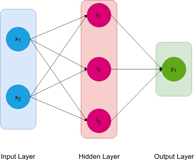
As the name suggests, SLFN is a neural net that has a single hidden layer. What makes them interesting is that they are simple, which makes them easier to understand, imagine, represent and reason about. We will start with a very simple example.

There are two neurons in the input layer, three in the hidden layer and one in the output layer. Usually, we are most concerned about the hidden layer and that is why this type of neural network is called single layer. By feedforward we mean that data during actual usage (not during training) flows only forward, from left to right. We can represent input to this network as a two dimensional vector $x \in R^{2}, x = [x_{1}, x_{2}]$, hidden layer as a three dimensional vector $l \in R^{3}, l = [l_{1}, l_{2}, l_{3}]$ and output simply as a number $y \in R, y = y_{1}$.
We will be more interested in connections, which are represented by arrows in the image. Every arrow represents weight of that connection. In order to calculate value $l_{1}$ we need to do the following:
\[l_{1} = g(x_{1} \cdot w_{11} + x_{2} \cdot w_{12} + b_{1})\]Let’s unpack this equation. $w_{11}, w_{12}$ are aformentioned weights connecting $x_{1}, x_{2}$ to to $l_1$ and $g$ is an activation function. If you do not know why bother with an activation function - it helps neural net learn learn complicated dependencies. You can read about this on this stackexchange post. What is $b_{1}$? It is a parameter called bias. It “moves” our function in proper direction if needed. My intuition goes as follows: We can have whole family of functions $x^{2} + b$, but in order to precisely identify which one I am talking about I need to pinpoint $b$ parameter which is a bias. In function $x^{2} + 4$, it is 4 that represent the bias. Now, with a little help of matrices we can write equation for j-th sample:
\(H_{j} = \begin{bmatrix} g(x_{j1} \cdot w_{11} + x_{j2} \cdot w_{12} + b_{1}) & g(x_{j1} \cdot w_{21} + x_{2} \cdot w_{22} + b_{2}) & g(x_{j1} \cdot w_{31} + x_{j2} \cdot w_{32} + b_{3}) \\ \end{bmatrix} \\ = \begin{bmatrix} g(\boldsymbol{x_{j}w_{1}} + b_{1}) & g(\boldsymbol{x_{j}w_{2}} + b_{2}) & g(\boldsymbol{x_{j}w_{3}} + b_{3}) \\ \end{bmatrix}\) Where bold dot mean vector dot product.
As you can see a connection between layers can be represented by a matrix.
So what is so extreme?
Now that we understand now SLFN look like we can get back to Extreme Learning Machines. The idea is simple - let’s assign a random value from continuous distribution (for people a little bit less math savvy, it’s just random), do the same for all values of the $w$ vector. After that, we can directly calculate the value of the matrix representing the second connection, which we will denote as $\hat{\beta}$.
Woah, that is a lot, so now it is time to unpack it.
Few lines above we have declared $H_j$ as a matrix representing hidden connection for a j-th sample. Matrix $H$ will represent hidden connections for all samples. Each row of the matrix will represent each sample. J-th label will be represented by $t_{j}$ and the whole vector with all labels will be denoted by $T$. The connection between the hidden and output layer will be denoted by $\hat{\beta}$ - it already represents connection for all the samples. For ELM it is also required that $g$ function is smooth, which for example - sigmoid is. Now we can write:
\[H\hat{\beta} = T\]And as we know H (it is random, but known) all we have to do is solve above matrix equation for $\hat{\beta}$.
To state it another way, we want to ensure that:
\[\Vert H\hat{\beta} - T = 0\Vert\]A more math-savvy person may see a problem with that approach. What if we have more samples then hidden neurons? Then we will have more equations than free variables, making this equation impossible to solve explicitly.
Enter the Moore–Penrose inverse
To tackle the above problem we can use Moore-Penrose inverse. It is a generalization of an inverse, sometimes called a pseudoinverse. There is a decent wiki article on this topic.
Moore-Penrose inverse provide least squares solution that also has minimal norm! That is exactly what we wanted.
Now, we can easily describe our algorithm:
- Assign random values to hidden weights and hidden biases
- Calculate the value of $H$
- Solve equation $H\hat{\beta} = T$ for $\hat{\beta}$
After dabbling ourselves a little bit in math, we should implement ELM. We will try to classify hand-written digit on MNIST dataset.
Sample Implementation on MNIST dataset
Jupyter notebook is available here